Computer Vision Model Architecture Guide: CNNs, YOLO, Vision Transformers, and VLMs in Production

Most computer vision write-ups stop at "we'll use a deep learning model." That's not a technical decision — it's a placeholder for one. The actual decision that determines whether a production system hits its latency budget, generalizes to real-world conditions, and stays maintainable a year in is which architecture family you pick, how you optimize it for your deployment target, and how you evaluate it against a metric that actually reflects your failure cost.

This is a technical reference, not a buyer's guide. It assumes you're the one making or reviewing the architecture decision, and it goes into the actual trade-offs: how CNN-based detectors, YOLO-family real-time models, transformer-based detectors, and foundation vision-language models differ under the hood, how to compress a model for edge deployment without destroying its accuracy, and how to measure whether any of it actually worked.

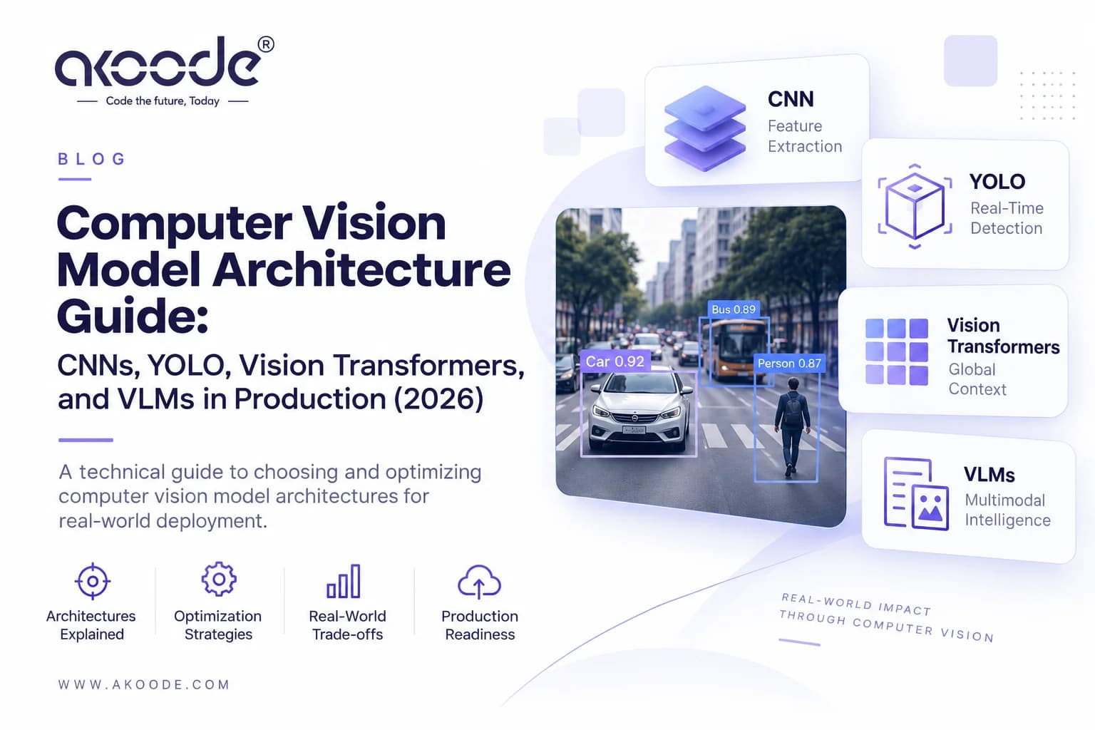
The Four Architecture Families, and What Actually Distinguishes Them

CNN-Based Detectors (Faster R-CNN, EfficientDet, and the two-stage lineage)

Two-stage detectors — a region-proposal network followed by a classification and refinement head — were the accuracy benchmark for years and still show up in applications where inference speed is secondary to precision: certain medical imaging pipelines, high-resolution industrial inspection where you can afford several hundred milliseconds per frame. The architectural cost is exactly what you'd expect from doing detection in two passes: proposal generation followed by classification is inherently slower than a single forward pass, which is precisely the constraint that motivated single-stage detection in the first place. Where two-stage CNN detectors still win: dense, small-object scenes (aerial imagery, cell counting in pathology slides) where the region-proposal step genuinely improves recall on objects a single-pass detector tends to miss.

YOLO-Family Single-Stage Detectors

The YOLO lineage reframed detection as a single regression problem — predict bounding boxes and classes directly from one forward pass — trading a small amount of accuracy for a large amount of speed, which is exactly the trade a real-time system needs. The family has moved fast: YOLO26, released by Ultralytics in early 2026, is the first version to natively unify detection, instance segmentation, classification, pose estimation, and oriented bounding box detection in one framework, and it removed two pieces of the classic pipeline — Non-Maximum Suppression (NMS) post-processing and Distribution Focal Loss — specifically to reduce inference latency variance and simplify edge deployment. NMS removal matters more than it sounds: NMS is a post-processing step whose runtime can vary based on how many overlapping boxes a frame produces, which makes worst-case latency unpredictable on exactly the kind of crowded scene (a factory floor, a retail aisle) where you need predictability most. An end-to-end, NMS-free design gives you a flatter, more predictable latency curve, which is what actually matters for a real-time SLA, not just average-case speed.

Where YOLO-family models fit: any scenario with a genuine real-time constraint and a reasonably fixed, known set of object classes — manufacturing defect detection, retail shelf monitoring, sports tracking, security camera analytics. They remain the default choice for edge deployment because the architecture was optimized for exactly that constraint from the ground up, not adapted to it after the fact.

Transformer-Based Detectors (DETR family, RT-DETR / RT-DETRv2)

Detection Transformers reframe the problem again — treating object detection as a set-prediction task solved with self-attention across the whole image, which removes the need for hand-designed anchor boxes and, in the end-to-end variants, removes NMS entirely by design rather than as a later optimization. RT-DETRv2 is the real-time-oriented branch of this lineage and is the most direct competitor to YOLO-family models in 2026: on standard object-detection benchmarks, the two architectures land in a similar accuracy range at comparable model sizes, but the underlying computation is fundamentally different — CNN-based efficiency in YOLO's case versus refined transformer attention in RT-DETR's case, which shows up in different latency profiles depending on hardware (GPU-heavy environments tend to favor transformer-based approaches more than CPU-constrained edge devices do, where the YOLO lineage's CNN backbone still tends to have the edge).

Where transformer detectors fit: scenes with complex spatial relationships between objects, cluttered scenes where anchor-based methods struggle, and deployments where you have GPU headroom to spend on attention computation rather than a tightly constrained edge device.

Foundation Vision-Language Models (CLIP-style embeddings, SAM-style segmentation, open-vocabulary detectors)

This is the category that's actually changed what "adding a new detection target" means. Instead of a fixed label set baked in at training time, foundation VLMs can be prompted with natural language — "flag any pallet blocking the emergency exit," "segment every scratch on this panel" — and generalize to concepts they weren't explicitly trained to detect as a discrete class. Under the hood, this usually means a vision encoder trained via contrastive learning against paired image-text data (the CLIP lineage), or a promptable segmentation model (the SAM lineage) that can be pointed at a region via a click, box, or text prompt rather than retrained per class.

The trade-off is real: open-vocabulary detection is generally slower and less precise on a narrow, well-defined task than a fine-tuned YOLO or RT-DETR model trained specifically for that task. Foundation VLMs earn their place when the actual problem is flexibility — a QA process that needs to detect a new defect type next month without a retraining cycle, or a security system that needs to respond to a novel, described condition rather than a pre-enumerated list of object classes.

Practical Read: Most Production Systems Now Combine Two of These

The single-architecture pitch is increasingly rare in serious builds. A common, effective pattern: a fast, fine-tuned YOLO or RT-DETR model handles the high-frequency, well-defined detection task in real time, while a foundation VLM sits downstream doing contextual reasoning on the detections it produces — "person" and "forklift" becomes "person within two meters of an active forklift" — without needing the reasoning layer to also carry the real-time detection load. Picking one architecture to do everything is usually a sign the trade-offs above weren't actually weighed.

A Decision Framework for Architecture Selection

Run through these five questions in order — each one materially narrows the field.

1. Is the class list fixed and known, or does it need to grow without retraining? Fixed and known → a fine-tuned YOLO or RT-DETR model. Needs to grow, or needs to handle natural-language-described conditions → a foundation VLM, likely combined with a fixed-class detector for anything that runs at high frequency.

2. What's the actual latency budget, and on what hardware? Sub-50ms on constrained edge hardware (no dedicated GPU) → YOLO-family, specifically a variant with NMS removed for predictable worst-case latency. GPU-available with more latency headroom → transformer-based detectors become competitive, and the accuracy gain may be worth the extra compute. For consumer mobile hardware specifically, running entirely on-device is often the more reliable path to a hard latency ceiling than optimizing a cloud round trip: Akoode's M2 Method pelvic health app needed corrective feedback within 300 milliseconds of a detected movement deviation, which was met by running pose estimation on-device using a pre-trained model rather than sending frames to a server at all — eliminating network latency from the budget entirely rather than trying to optimize it down.

3. How much labeled data do you actually have? Small dataset, hard to grow → lean on a pretrained foundation model fine-tuned with few-shot or transfer learning rather than training a detector from scratch, which needs substantially more labeled data to converge well. Larger, well-curated dataset → a from-scratch or heavily fine-tuned YOLO/RT-DETR model will generally outperform a generalist foundation model on the narrow task.

4. Do you need more than bounding boxes — segmentation, pose, oriented boxes? Multi-task requirements point toward the newer unified frameworks (YOLO26's multi-task design is built for exactly this) rather than stitching together separate single-purpose models, which multiplies your maintenance burden for a marginal accuracy gain.

5. What does the failure cost actually look like? If false negatives are catastrophic (a missed structural defect, a missed safety violation), that changes not just which metric you optimize for (recall over raw accuracy — more on this below) but potentially which architecture: two-stage CNN detectors' stronger performance on small, easy-to-miss objects can be worth the latency cost when a miss is expensive enough.

Optimizing a Model for Deployment

Picking the right architecture family is half the job. The other half is making it run efficiently in its actual deployment environment, which for anything edge-based usually means active compression, not just exporting the trained model as-is.

Quantization. Reducing numerical precision — typically from 32-bit floating point down to 16-bit or 8-bit integers — shrinks model size and speeds up inference, often substantially, with a real but usually small accuracy cost if done carefully. Post-training quantization is faster to apply but riskier on accuracy; quantization-aware training, where the model learns to tolerate reduced precision during the training process itself, generally preserves more accuracy at the cost of a longer training cycle. INT8 quantization is the common target for CPU-only edge devices; FP16 is often sufficient when a mobile GPU or NPU is available. Akoode's Sahayak Diagnostic Orchestrator, a dual-stream clinical decision support system for cervical spine and chest pathology detection, is a useful concrete example of this trade-off working out well: mixed-precision (FP16) inference on NVIDIA T4 GPU hardware cut a full study's processing time to roughly 41 milliseconds without reducing detection accuracy — the alternative, simplifying the model architecture to hit that speed, would have cost exactly the accuracy the clinical use case couldn't spare.

Pruning. Removing weights or entire channels that contribute little to the model's output, based on magnitude or sensitivity analysis, reduces both model size and compute. Structured pruning (removing whole channels or layers) tends to translate into real inference speedups on standard hardware; unstructured pruning (removing individual weights) often achieves higher theoretical sparsity but needs specialized hardware or software support to realize an actual speed benefit — a common gap between benchmark numbers and real deployment gains.

Knowledge distillation. Training a smaller "student" model to mimic the output behavior of a larger, more accurate "teacher" model transfers much of the teacher's accuracy into a model small and fast enough for constrained hardware. This has become common enough that it now shows up as a built-in training option in several production frameworks rather than a bespoke research technique — a sign of how standard the technique has become for edge deployment specifically.

Export format and runtime. The trained model needs to leave its training framework and run in a production-optimized runtime — ONNX Runtime for cross-platform deployment, TensorRT for NVIDIA hardware specifically, Core ML for Apple devices. Each conversion step is a place accuracy can silently shift if operations aren't supported identically across frameworks, which is why a validation pass after export — not just after training — is a step serious teams don't skip.

NMS-free architectures reduce a whole class of edge deployment pain. Because traditional NMS post-processing runs at variable cost depending on scene density, it's historically been one of the harder pieces to optimize and export cleanly to edge runtimes. Architectures built without it (YOLO26 and the DETR lineage generally) sidestep that specific optimization problem entirely, which is part of why the industry has been moving in that direction for edge-targeted work.

Evaluation Metrics: Why a Single Accuracy Number Doesn't Tell You Anything

"95% accurate" is close to meaningless in isolation for a detection task, and a vendor or team that leads with it without qualification hasn't finished the analysis. Here's what actually needs to be reported, and why each matters:

• Precision — of everything the model flagged, what fraction was actually correct. Low precision means excessive false alarms, which matters enormously in something like a security system generating alert fatigue.

• Recall — of everything that should have been flagged, what fraction the model actually caught. Low recall means missed detections, which matters enormously in something like a defect-detection line or a diagnostic imaging tool, where a miss is the expensive failure mode.

• F1 score — the harmonic mean of precision and recall, useful as a single number only when false positives and false negatives cost roughly the same, which is rarely true — most real deployments should pick a threshold that favors whichever error type is more expensive, not the mathematically balanced point.

• IoU (Intersection over Union) — for detection and segmentation, how well a predicted bounding box or mask overlaps the ground truth. The IoU threshold used to count a detection as "correct" (commonly 0.5, sometimes stricter) materially changes reported accuracy, which is why mAP is always reported against a specific threshold or range.

• mAP (mean Average Precision) — the standard detection benchmark metric, averaged across classes and often reported at a single IoU threshold (mAP@50) or averaged across a range of thresholds (mAP@50-95, the stricter and more informative version). A model that looks strong at mAP@50 but drops sharply at mAP@50-95 is producing boxes that are roughly right but not precisely right — worth knowing before it matters in production.

• Calibration — whether a model's confidence scores actually correspond to real-world correctness rates. An overconfident model (reporting 95% confidence on detections that are only right 70% of the time) makes downstream decision thresholds unreliable, and calibration is frequently skipped in production evaluation even though it directly affects how safely a system's output can be automated on.

The practical rule: agree on the metric that matches your actual cost of failure before training starts, not after results come in, and report it broken down by class — an aggregate number hides the fact that a model can be excellent on common classes and nearly useless on the rare, high-stakes one. Sahayak's reporting reflects this discipline in practice: spine fracture detection and chest pathology classification are reported as two separate accuracy figures (99.1% and 98.4% respectively) rather than one blended number, because they're different tasks with different failure costs, and each is paired with Grad-CAM attention maps so a clinician can see exactly which region of the image drove a given classification — the calibration and trust problem solved visually rather than left as an unexplained confidence score.

Data Engineering: The Part That Determines Whether Any of This Works

Active learning loops. Rather than annotating data randomly, prioritize labeling the frames the current model is least confident about or gets wrong most often. This concentrates annotation effort where it actually moves accuracy, which matters because annotation budget is almost always the real constraint, not model architecture.

Class imbalance handling. Real-world defect rates, rare safety events, and uncommon object classes mean training data is almost never balanced. Techniques like focal loss (which down-weights the contribution of easy, well-classified examples during training so the model focuses on hard and rare cases) and targeted oversampling of minority classes are standard responses — a vendor who hasn't discussed how they'll handle this on a genuinely imbalanced dataset hasn't scoped the problem correctly. The Sahayak diagnostic system faced this directly: medical imaging datasets skew heavily toward healthy scans, which trains models that are good at confirming health and poor at catching pathology. The response there was a two-phase fine-tuning strategy specifically designed to prevent the pre-trained backbone's weights from shattering during adaptation, combined with CLAHE contrast enhancement in preprocessing to improve sensitivity on the lower-contrast inputs where subtle pathology is easiest to miss.

Synthetic data generation. For rare edge cases that are expensive or slow to collect naturally — an unusual defect type, a rare lighting condition, a low-frequency safety event — generating realistic synthetic training examples (via simulation, generative models, or domain randomization) can close a coverage gap that would otherwise take months of real-world data collection to fill.

Annotation quality control. Inter-annotator agreement — how consistently multiple human labelers agree on the same image — is a leading indicator of dataset quality that gets skipped surprisingly often. A dataset with low agreement on ambiguous cases will produce a model that's confidently wrong on exactly the cases that matter most, because it learned from inconsistent ground truth.

Production Monitoring: Detecting Drift Before It Becomes an Incident

A model's accuracy at launch is a snapshot, not a guarantee. Camera hardware gets swapped, lighting shifts seasonally, a product line changes — all of which can silently degrade a model that was validated correctly at deployment. The technical methods that catch this before someone notices from the output:

Population Stability Index (PSI) and distributional monitoring. Comparing the statistical distribution of incoming production data (pixel intensity distributions, detected object size distributions, class frequency) against the distribution the model was trained on. A rising PSI score signals the input data is drifting away from what the model was validated on, often before accuracy visibly drops.

Confidence score monitoring. Tracking the distribution of the model's own confidence scores over time. A gradual downward shift, or a growing cluster of low-confidence predictions, is often the earliest visible signal of drift — well before ground-truth labels (which are often delayed or expensive to obtain in production) confirm an actual accuracy drop.

Embedding-space drift detection. For models built on learned feature embeddings, monitoring how the distribution of embeddings for production inputs shifts relative to the training distribution can catch subtler forms of drift that raw input statistics miss — a scene composition change that doesn't show up in pixel-level stats but does show up in how the model internally represents the input.

Shadow deployment and canary rollout for retrained models. When a model is retrained to address detected drift, deploying it in shadow mode (running alongside the production model without its output being acted on, purely for comparison) or as a canary (serving a small percentage of live traffic) catches regressions before a full rollout, rather than discovering a problem after every prediction is already routed through the new model.

A production computer vision system without at least the first two of these running is not a monitored system — it's a system that will eventually surprise someone.

Four Architecture Decisions From Production: What Actually Got Built

Computer Vision Architecture Decision Tree

                         Computer Vision Problem
                                  │
                    ┌─────────────┴─────────────┐
                    │                           │
              Fixed Classes?              Open Vocabulary?
                    │                           │
                   Yes                          Yes
                    │                           │
                    ↓                           ↓
              YOLO / RT-DETR             VLM / Foundation
                    │                           │
             ┌──────┴──────┐                    │
             │             │                    │
          Edge CPU      GPU / NPU        Hybrid Pipeline
             │             │                    │
             └──────┬──────┘                    │
                    │                           │
                    └─────────────┬─────────────┘
                                  ↓
                       Production Deployment
                                  │
                    ┌─────────────┴─────────────┐
                    │                           │
              Low Latency                  High Reasoning
                    │                           │
                    ↓                           ↓
             Optimized CV Model          VLM / Hybrid Model
                    │                           │
                    └─────────────┬─────────────┘
                                  ↓
                       Monitor & Optimize

The right architecture depends on the actual production requirement. Fixed-class, real-time detection often favors optimized models such as YOLO or RT-DETR, while open-vocabulary and reasoning-heavy use cases may benefit from vision-language or foundation models. In many production systems, a hybrid architecture provides the best balance between speed, accuracy, and reasoning capability.

Production Computer Vision Pipeline

                         Camera / Image
                               │
                               ↓
                       Pre-processing
                               │
                               ↓
                        Detection Model
                               │
                               ↓
                    Tracking / Segmentation
                               │
                               ↓
                         VLM / Reasoning
                               │
                               ↓
                         Business Rules
                               │
                    ┌──────────┴──────────┐
                    │                     │
                    ↓                     ↓
              Alert / Action         API / Dashboard
                    │                     │
                    └──────────┬──────────┘
                               ↓
                    Monitoring & Analytics
                               │
                               ↓
                     Feedback / Retraining
                               │
                               └──────────────┐
                                              │
                                              ↓
                                      Model Optimization
                                              │
                                              └──────→ Production

A production computer vision system is rarely just a model. The complete pipeline typically includes image preprocessing, detection, tracking or segmentation, reasoning, business logic, application integration, monitoring, and continuous optimization.

Computer Vision Architecture Comparison

Choosing the Right Architecture

There is no universally "best" computer vision architecture. The right choice depends on factors such as:

• Latency requirements — How quickly must the system respond?

• Accuracy requirements — What level of precision and recall is acceptable?

• Hardware constraints — Will the model run on an edge CPU, GPU, NPU, or cloud infrastructure?

• Object and scene complexity — Are the classes fixed or open-ended?

• Dataset availability — How much labeled training data is available?

• Reasoning requirements — Does the system only need to detect objects, or also interpret and reason about visual context?

• Deployment scale — Will the system process one camera or thousands of concurrent streams?

• Maintenance requirements — How frequently will the model need retraining or optimization?

For simple, fixed-class real-time detection, an optimized YOLO-based architecture may be the most practical choice. For more complex applications requiring open-ended visual understanding, a VLM or hybrid architecture may be more appropriate.

The goal is not to choose the most sophisticated model. The goal is to choose the architecture that delivers the required accuracy, latency, cost, reliability, and maintainability in the target production environment.

Every trade-off above sounds cleaner on paper than it plays out in a real build. Four Akoode projects illustrate how these decisions actually get made once real constraints are in the room, each shaped by a different binding constraint: raw latency, data residency, clinical accuracy under class imbalance, and on-device inference on consumer hardware.

Real-time multi-object tracking under a hard latency budget. A professional American football coaching organization needed player tracking across up to 15 simultaneous 4K camera feeds at 60fps, with results delivered the same day footage was captured — not after a multi-day manual review cycle. That combination of constraints (high resolution, many parallel streams, a same-day turnaround requirement) ruled out a two-stage CNN detector immediately on latency grounds and pointed toward a real-time single-stage architecture, with the actual engineering weight falling on the tracking and re-identification layer, not the detector itself: keeping a consistent identity on each player through constant collisions and overlap is the harder problem once detection alone is fast enough. The system was built on a GPU-accelerated streaming pipeline processing every camera feed in parallel, with training data deliberately augmented across a wide range of lighting conditions since the system had to hold up across different stadiums and match conditions, not one clean baseline. It now runs at 94% multi-player tracking accuracy across play types, including high-speed movement and full-contact collisions — the full case study covers the tiered storage architecture used to keep the resulting data volume manageable.

Document-based detection with a hard no-cloud constraint. Qualis Construction Ltd., a Canadian estimating firm, needed an AI quantity takeoff platform to detect materials, fixtures, and measurements directly from architectural and engineering drawings — work that used to consume hours of manual measurement per project. The deciding architecture constraint here wasn't latency, it was data sensitivity: architectural drawings routinely contain proprietary project information that can't leave the client's environment, which made offline, on-premise processing a hard requirement rather than a preference. That single constraint shapes the entire model choice differently than the sports-tracking build above — instead of optimizing purely for real-time throughput across streaming video, the priority becomes a model efficient enough to run reliably without cloud inference, deployed against static, information-dense documents rather than fast-moving video frames. It's a useful contrast case for the decision framework above: two computer vision problems, two entirely different binding constraints, two different architecture paths. The full case study has the detail.

Volumetric sequence modeling for a clinical accuracy floor. The Sahayak Diagnostic Orchestrator, built as a dual-stream clinical decision support system, needed to detect cervical spine fractures across C1 through C7 and classify chest pathologies from X-rays at specialist-comparable accuracy, fast enough to triage a busy emergency radiology worklist. The architecture decision that mattered most here wasn't the detection backbone alone — standard models reading each CT slice as an independent 2D image miss fractures that span multiple vertebral levels, so a hybrid EfficientNetV2-B3 feature extractor was paired with Bidirectional GRU units to read the spine as a continuous anatomical sequence rather than flat slices. Combined with the two-phase fine-tuning and mixed-precision optimization described earlier, the system reports 99.1% spine accuracy and 98.4% chest accuracy with a 41-millisecond inference time and Grad-CAM explainability on every finding. The full case study covers the triage and clinical interface layer built on top of the model.

On-device pose estimation for a therapeutic feedback loop. M2 Method needed a validated Python pose-detection proof of concept turned into a production mobile app delivering real-time corrective feedback for pelvic floor rehabilitation exercises — a domain where a slow or wrong correction carries real clinical risk, not just a poor user experience. The architecture decision was to keep pose estimation entirely on-device using a pre-trained model mapping 33 body landmarks per frame, paired with a JSON-configurable rule engine comparing calculated joint angles against exercise-specific biomechanical thresholds, rather than retraining a custom detector or relying on any server round trip. That combination met a 300-millisecond feedback ceiling on standard consumer smartphones. The full case study covers the rebuild from desktop OpenCV prototype to production Flutter application.

The pattern worth taking from all four: none of these projects started with "which model architecture." Each started with the one non-negotiable constraint — a latency SLA, a data-residency requirement, a clinical accuracy floor on imbalanced data, or a feedback deadline on consumer hardware — and let that constraint eliminate most of the architecture space before accuracy benchmarks even entered the conversation.

Frequently Asked Questions

Should I choose YOLO or a vision transformer for object detection?

For real-time, edge-constrained deployment with a fixed set of object classes, YOLO-family models generally remain the stronger default because the architecture was built around exactly that constraint. Transformer-based detectors like RT-DETRv2 become more competitive when GPU headroom is available and scene complexity (cluttered, overlapping objects) benefits from attention-based reasoning across the whole image.

What's the actual benefit of removing NMS from a detection model?

Non-Maximum Suppression is a post-processing step with runtime that varies based on how many overlapping detections a frame produces, which makes worst-case latency unpredictable on crowded scenes. NMS-free, end-to-end architectures produce a flatter, more predictable latency profile — which matters more for a real-time SLA than average-case speed alone.

When does a foundation vision-language model make more sense than a fine-tuned detector?

When the detection target needs to change without a retraining cycle — a QA process adding a new defect description, a security system responding to a novel described condition — or when labeled training data for the specific task is too scarce to fine-tune a dedicated detector effectively.

What's the difference between quantization and pruning?

Quantization reduces the numerical precision used to represent model weights and activations (commonly from 32-bit floating point to 8-bit integers), shrinking size and speeding up inference. Pruning removes weights, channels, or layers that contribute little to the model's output. They're complementary and often applied together for edge deployment.

Why does mAP@50-95 matter more than mAP@50?

mAP@50 only requires a predicted bounding box to overlap the ground truth by 50% to count as correct — a fairly loose bar. mAP@50-95 averages performance across a range of stricter overlap thresholds, which better reflects whether a model produces boxes that are precisely, not just roughly, correct — important for any downstream use that depends on accurate localization, not just detection.

How do you detect model drift before it shows up in accuracy metrics?

Monitor the statistical distribution of incoming production data against the training distribution (via a metric like Population Stability Index) and track the model's own confidence score distribution over time. Both tend to shift before ground-truth-confirmed accuracy drops become visible, since ground truth in production is often delayed or expensive to collect.

Do I need a different model architecture for segmentation versus detection?

Not necessarily anymore. Newer unified frameworks (YOLO26 among them) natively support detection, segmentation, classification, pose estimation, and oriented bounding boxes within one architecture, which is generally preferable to maintaining separate single-purpose models unless a narrow, specialized model meaningfully outperforms the unified option on your specific task.

Where This Fits at Akoode

This architecture and optimization layer is the engineering core underneath the systems covered in our broader look at computer vision architecture and industry use cases — including the four production builds referenced above: real-time multi-camera player tracking, offline document-based detection for construction estimating, volumetric medical imaging analysis, and on-device pose correction for mobile. Between them they cover most of the constraint space this guide walks through — latency-bound real-time video, data-residency-bound static documents, clinical accuracy under class imbalance, and consumer-hardware edge inference. If you're evaluating a computer vision partner rather than building in-house, our vendor evaluation guide covers what to ask.

Akoode's AI development work — including computer vision systems built around exactly this kind of architecture and deployment decision-making — holds a 4.9 Google rating from 110+ reviews and a 5.0 out of 5 on GoodFirms. For a technical scoping conversation if you are Building a Computer Vision System for Production?

Choosing the right model is only the beginning. The real challenge is building a computer vision system that delivers the right balance of accuracy, latency, scalability, cost, and reliability in production.

Akoode Technologies helps businesses design and deploy production-ready computer vision solutions—from architecture selection and model optimization to edge deployment, cloud infrastructure, real-time inference, and AI-powered workflows.

Whether you're starting a new computer vision project or optimizing an existing system, our team can help you identify the right architecture and build a practical path to production.

→ Discuss Your Computer Vision Architecture with Akoode Technologies